

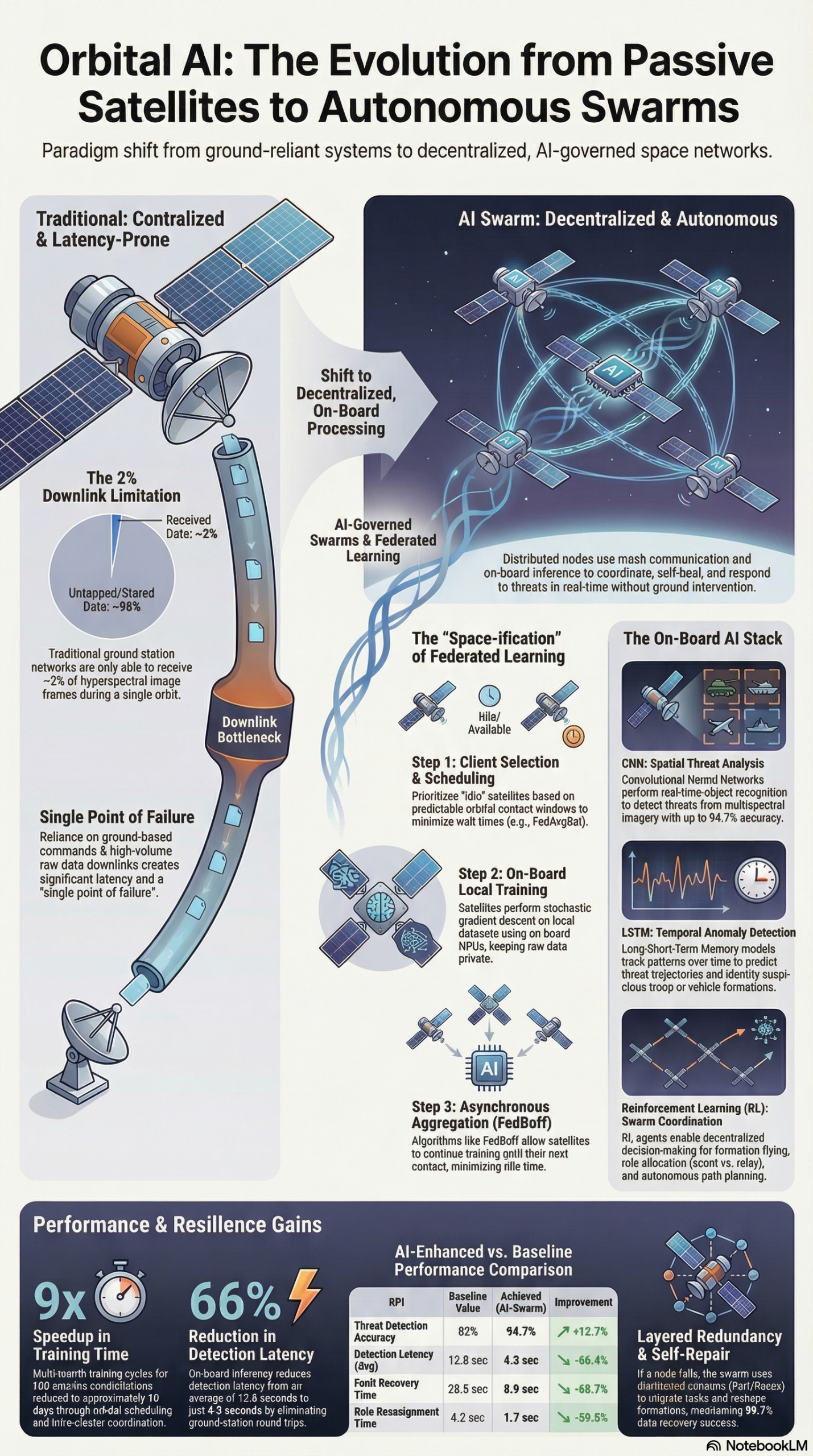
Satellite constellations are drowning in data they cannot transmit — Landsat-8 alone generates over 400 TB of imagery annually, yet ground stations capture only about 2% of hyperspectral frames per orbit. The fix is not more bandwidth. It is moving the intelligence onboard, using Federated Learning and autonomous AI swarms to process data where it lives. This tutorial walks through the complete architecture, algorithm selection, hardware configuration, and deployment decisions required to build a distributed orbital ML pipeline.
What This Is
Federated Learning Meets Low Earth Orbit
Federated Learning (FL) is a distributed machine learning paradigm where nodes train models locally on their own data and share only model weight updates — never raw data — with a central aggregator. In terrestrial applications, this is already deployed at scale across millions of smartphones without centralizing sensitive data. In space, it addresses an even more acute problem: the downlink bottleneck.
According to the NotebookLM research report, modern high-resolution Earth observation missions like Landsat-8 produce over 400 TB of data annually, but ground station contact windows last only 5–15 minutes per orbit. During that window, a satellite can transmit only a fraction of what it has captured. At constellation scale — where hundreds or thousands of spacecraft are continuously imaging the Earth — this becomes a critical operational gap. The constellation is effectively blind to most of what it observes, with imagery sitting on onboard storage until the next downlink opportunity hours or days later.
The solution documented in the research is the “space-ification” of FL: adapting established terrestrial algorithms (FedAvg, FedProx, FedBuff) to work within the hard constraints of orbital mechanics. This requires three fundamental changes from terrestrial FL implementations, as outlined in the research report:
- Client selection based on which satellites are first to make ground contact, replacing the random sampling used in terrestrial FL
- Round completion synchronized to deterministic orbital revisit times, not wall-clock intervals
- Asynchronous buffering via FedBuffSat to minimize satellite idle time between contact windows
The most significant variant introduced for space operations is FedBuffSat, which implements a “bounded staleness” approach. This allows satellites to continue local training and contribute model updates at their next contact window rather than waiting for all nodes to synchronize globally. This is not just an optimization — it is architecturally necessary when satellites have 90-minute orbital periods and only 10-minute windows to transmit.
Two modular enhancements build on top of the space-ified base algorithms, as documented in the research report:
FLSchedule (Orbital Scheduling): Precomputes satellite orbits to prioritize clients with the shortest combined initial contact time and revisit time. This physics-based client selection reduces total round duration and satellite idle time by nearly half compared to unoptimized orbital FL.
FLIntraCC (Intra-Cluster Communication): Uses intra-satellite links (ISLs) to relay model updates through peers within the same orbital cluster. This enables satellites without direct ground contact to contribute their model updates through cluster members that do have contact — dramatically increasing participation rates per FL round.
Beyond Earth observation, this same distributed architecture extends to autonomous AI swarms for national defense applications. These swarm systems deploy Convolutional Neural Networks (CNN) for spatial object recognition and Long Short-Term Memory (LSTM) networks for temporal anomaly detection, running onboard with inference latency under 1.3 seconds. The swarm operates as a dynamic graph of cooperating agents governed by Multi-Agent Reinforcement Learning (MARL), enabling decentralized coordination without any ground command dependency, as the research report documents in detail.
The implications extend beyond any single mission. As the research states: “As LEO satellite constellations rapidly expand to hundreds and thousands of spacecraft, the need for distributed on-board machine learning becomes critical to address downlink bandwidth limitations.” The infrastructure for mega-constellations like Starlink and Project Kuiper is being deployed now. The data management crisis is not a future problem.
Why It Matters
From Passive Observers to Intelligent Orbital Networks
The traditional satellite operations model is simple: observe, store, downlink, analyze on the ground. It functioned when constellations had a handful of spacecraft and Earth observation was a niche scientific endeavor. Today, that model collapses under its own data weight.
The research report puts the strategic problem plainly: “Traditional satellite systems are predominantly passive, centralized, and reliant on ground-based commands. These constraints render such systems suboptimal in scenarios requiring agility, redundancy, and autonomous response.” Ground-based latency introduces delays that are unacceptable in real-time applications — disaster response, maritime domain awareness, tactical surveillance. A satellite that must wait for a downlink window, ship raw data to a ground processing center, run inference there, and then wait for commands to be uplinked back is operating on a 4–6 hour action loop at minimum. With onboard FL and swarm intelligence, that loop collapses to minutes.
Who benefits, specifically:
Commercial Earth Observation operators running constellations for agriculture, insurance, or climate monitoring can dramatically increase the cadence at which useful ML models are trained and deployed across their fleets. A 9x speedup in training cycles — from multi-month cycles down to approximately 10 days — means faster model updates for crop health monitoring, flood extent mapping, and infrastructure change detection without expanding ground infrastructure.
Defense and intelligence agencies gain persistent surveillance capability that does not depend on ground infrastructure that can be jammed, destroyed, or simply unavailable in contested environments. Swarm redundancy, backed by Reed-Solomon erasure coding, ensures that losing 40% of nodes does not compromise mission continuity, as documented in the research report.
Mission designers and satellite system architects now have a documented, tested framework for deploying distributed ML rather than building bespoke solutions from scratch. FLSchedule and FLIntraCC provide validated, modular components that can be integrated into constellation design during the architecture phase — where they cost nothing to include but everything to retrofit.
Hardware developers building AI-capable edge chips for space applications have reference architectures — AMD Versal AI Edge, NVIDIA Jetson Nano, RK3588 — validated specifically for orbital ML inference.
The commercial cost structure implication is significant: instead of designing constellations around maximizing downlink bandwidth (expensive ground station infrastructure, inter-satellite laser links primarily for communication throughput), operators can design around maximizing onboard compute and local learning. This is a fundamentally different optimization target with different cost curves.
The Data
FL Performance Benchmarks and Swarm Architecture Specifications
The research report provides concrete performance data on both the FL training pipeline and the swarm architecture. The tables below summarize key figures from that analysis.
Federated Learning Performance — Baseline vs. Optimized:
| Metric | Unoptimized Orbital FL | With FLSchedule + FLIntraCC | Source |
|---|---|---|---|
| FL Training Duration | Multi-month cycles | ~10 days | Research Report |
| Speedup Factor | 1x | 9x | Research Report |
| Per-Round Duration Reduction | Baseline | ~50% reduction | Research Report |
| Optimal Ground Station Count | Variable | ~5 globally distributed | Research Report |
| Hyperspectral Frame Utilization | ~2% per orbit | Increased via onboard inference | Research Report |
| Annual Data Volume (Landsat-8 scale) | 400+ TB raw downlink | Bandwidth reduced to weight updates | Research Report |
Swarm AI Architecture Technical Specifications:
| Component | Technical Detail | Source |
|---|---|---|
| Onboard Inference Latency | ≤1.3 seconds per frame | Research Report |
| CNN Object Detection Precision | 91.4% | Research Report |
| Fault Recovery Protocol | Raft or Paxos for leader election | Research Report |
| Data Integrity (Node Loss Tolerance) | Reed-Solomon; survives 40% node loss | Research Report |
| Consensus Mechanism | Bounded-delay synchronous gossip | Research Report |
| Security Protocol | Post-Quantum Cryptography (PQC) | Research Report |
| Audit Trail | Blockchain-based tamper-proof log | Research Report |
| Reference Hardware | NVIDIA Jetson Nano, RK3588, AMD Versal AI Edge | Research Report |
Step-by-Step Tutorial
Building an Orbital Federated Learning Pipeline from Architecture to Deployment
This walkthrough covers the architecture decisions, algorithm selection, hardware configuration, and validation steps for deploying a federated learning system across a LEO satellite constellation. These are system-design decisions — the choices made here determine whether your system converges in 10 days or produces a divergent model that never ships.
Prerequisites
Before beginning constellation FL design, confirm you have:
- A defined constellation topology: satellite count, orbital altitude, inclination angles, and planned cluster structure
- Onboard compute specification: at minimum a capable CPU with 2+ GB RAM; for production ML inference, a dedicated NPU or GPU SoC such as AMD Versal AI Edge, NVIDIA Jetson Nano, or RK3588
- Ground station access plan: at least 3–5 globally distributed stations, including polar facilities for polar-orbiting constellations
- A defined ML task with a validated dataset: object classification, anomaly detection, and change detection are the most extensively documented use cases for orbital FL
- Baseline familiarity with FedAvg or FedProx as aggregation algorithms before implementing space-specific variants
Phase 1: Topology Analysis and Cluster Architecture
The single most important design decision in orbital FL is cluster structure. The research report is unambiguous: intra-cluster density is more effective at reducing FL training time than total constellation size. A tightly-spaced cluster of 12 satellites in the same orbital plane will outperform a dispersed constellation of 50 satellites for FL convergence, because co-orbital satellites can leverage sequential ground station access and ISL-based data relay within the cluster.
Step 1: Define your orbital clusters. Group satellites by orbital plane. Satellites sharing an orbital plane have predictable, stable relative geometries that simplify ISL geometry and contact window modeling. Assign each cluster an initial “relay candidate” — the satellite expected to have the shortest combined initial contact time and revisit time to your primary ground stations. This assignment will be updated dynamically by FLSchedule at runtime, but a static initial mapping is needed for link budget analysis.
Step 2: Model ground station contact windows. Run orbital mechanics simulations using STK, GMAT, or the open-source Orekit library to compute precise contact windows for each satellite across each ground station. The outputs you need are: for each satellite in each orbital cluster, the timestamp of its next contact window, the window duration, and its revisit period. This data feeds directly into FLSchedule’s precomputation step. Notably, the research report shows that FL performance gains plateau after approximately five globally distributed ground stations — additional stations beyond that threshold yield diminishing returns on round duration reduction.
Step 3: Prioritize polar ground station placement. For polar-orbiting constellations, high-latitude ground stations — such as those at Tromsø, Norway or facilities in Alaska and Svalbard — see nearly every satellite in the constellation multiple times daily. Positioning your primary FL aggregation function at these stations maximizes round throughput far more than adding mid-latitude stations. As the research report recommends: optimize ground station placement over quantity.
Phase 2: Algorithm Selection and Space-ification
Step 4: Choose your base aggregation algorithm based on contact window regularity. For constellations with predictable, regular contact windows, FedAvg provides the simplest baseline. For constellations with irregular access patterns or heterogeneous data distributions across satellites, FedProx adds a proximal regularization term that prevents model divergence when individual satellite updates drift far from the global model. For large constellations where maximizing throughput is paramount, implement FedBuffSat — the asynchronous buffer variant specifically designed for orbital FL. FedBuffSat is the production-grade choice for any constellation with more than 20 satellites.
Step 5: Configure bounded staleness in FedBuffSat. Bounded staleness is the architectural core of FedBuffSat: model updates from satellites trained N rounds ago are accepted, not discarded. Set your staleness bound based on your orbital period and contact window frequency. For a typical 90-minute LEO orbit with 12-hour revisit periods, a staleness bound of 2–4 rounds prevents both excessive data aging and satellite idle time. Set the bound too tight and you recreate the synchronous blocking problem you were trying to avoid. Set it too loose and you introduce accuracy degradation from stale gradient updates. Tune this empirically against your specific constellation geometry and task, not from a default template.
Step 6: Enforce minimum local epoch requirements per satellite. When FLSchedule aggressively optimizes round duration by shortening contact windows, individual satellites have less wall-clock time for local training. The research report explicitly flags this: enforce a minimum number of local training epochs per satellite per round. Satellites that contribute underfit model updates — because they ran only 1–2 epochs before their contact window closed — actively degrade the global model. A practical floor is 3–5 local epochs per round for typical Earth observation classification tasks. Test your chosen floor against a convergence curve before finalizing.
Phase 3: Intra-Cluster Communication with FLIntraCC
Step 7: Enable intra-satellite links for model update relay. FLIntraCC allows satellites that lack a direct ground contact window to relay their model weight updates through cluster peers that do have contact. Without this, satellites on the far side of an orbit during a given FL round simply miss that round, reducing effective cluster participation and slowing convergence. ISLs are the physical mechanism — optical or RF inter-satellite links that cluster members maintain with their nearest neighbors in the same orbital plane.
Step 8: Assign relay responsibilities dynamically by orbital geometry. At each FL round, the cluster member with the next scheduled ground contact becomes the relay aggregator for that round. Other cluster members without direct contact transmit their weight update packages via ISL to the designated relay node, which downlinks the bundle. Configure your ISL link management software to handle relay role transitions automatically as the orbital geometry changes. Static relay assignments fail as soon as any satellite misses a contact window.
Step 9: Allocate dedicated ISL bandwidth for FL relay traffic. Model update relay via ISL consumes link budget. When designing the ISL link budget for your constellation, allocate a dedicated traffic class for FL weight update relay that cannot be preempted by other ISL uses (telemetry, command, primary mission data relay). A typical CNN weight update delta for a mid-size classification model is 1–10 MB. At 12 satellites per cluster with 10-minute contact windows, the required FL relay bandwidth is modest — but it must be guaranteed, not best-effort.
Step 10: Stress-test FLIntraCC with simulated contact failures. Before finalizing your architecture, run simulations where 30% of satellites miss their scheduled contact windows per round — equipment faults, atmospheric conditions, and scheduling conflicts are realistic causes. Measure the accuracy of the global model under these degraded conditions. If accuracy degrades more than your mission tolerance allows, either increase cluster density or add redundant relay paths within the cluster topology.
Phase 4: Swarm Intelligence Integration for Real-Time Surveillance
For constellations requiring autonomous coordination and real-time threat detection beyond FL model training, integrate the swarm AI architecture documented in the research report.
Step 11: Deploy the CNN + LSTM inference stack onboard. The swarm architecture uses CNNs for spatial object detection — identifying tanks, ships, aircraft, or infrastructure — and LSTMs for temporal anomaly detection, tracking movement vectors across multiple satellite passes over time. Per the research report, the CNN component achieves 91.4% detection precision. Deploy these as separate inference modules on your onboard NPU, optimized for the AMD Vitis AI toolchain targeting the Versal AI Edge SoC. Run the two models in a pipeline: CNN outputs per-frame detections, LSTM ingests the detection sequence to flag anomalous movement patterns.
Step 12: Implement the MARL coordination layer. Multi-Agent Reinforcement Learning governs the swarm’s task allocation, formation maintenance, and autonomous recovery from node failures. Each satellite runs a local RL policy that takes local sensor observations and peer state information (received via gossip protocol over ISLs) as inputs, and outputs coordination actions — sensor pointing commands, data relay decisions, and role assignments within the swarm hierarchy. The swarm topology is modeled as a dynamic undirected graph G = (V, E), where edges represent active ISL connections between nodes. When a node goes offline, the graph re-forms around the surviving nodes via the consensus protocol.
Step 13: Configure the security and consensus stack. Defense deployments require Post-Quantum Cryptographic (PQC) protocols on all inter-satellite and downlink communications, as documented in the research report. Implement Raft or Paxos for federated leader election — when a designated “Leader” or “Tracker” satellite fails, the surviving swarm nodes elect a replacement autonomously via the consensus protocol without waiting for a ground command. Configure Reed-Solomon erasure coding to tolerate the loss of up to 40% of swarm nodes without losing observation data. Establish the blockchain-based audit log at commissioning, not as an afterthought — it is the chain-of-custody mechanism for intelligence products and must be initialized before operational data collection begins.
Phase 5: Hardware Deployment on AMD Vitis AI
Step 14: Set up the AMD Vitis AI development environment. AMD Vitis AI provides quantization tools and NPU (Neural Processing Unit) IP for Versal AI Edge Series SoCs, as noted in the research report. Pull the official Vitis AI Docker image from AMD’s repository. Configure the DPU (Deep Processing Unit) IP for your target Versal device variant. Load your trained PyTorch or TensorFlow models — Vitis AI accepts both — as the starting point for the quantization workflow.
Step 15: Quantize and compile models for onboard deployment. Use the Vitis AI quantizer to convert your CNN and LSTM models from 32-bit floating point to INT8 precision. This step is non-negotiable for space deployment: INT8 quantization reduces model memory footprint by 4x and inference compute by 2–4x compared to FP32, which directly determines whether your model fits within the power envelope of a space-qualified SoC. Compile the quantized models for the DPU architecture. Target inference latency should be ≤1.3 seconds per frame for real-time surveillance applications, as benchmarked in the research report. Validate quantized model accuracy against your full-precision baseline before signing off — INT8 quantization on well-trained models typically loses less than 1–2% task accuracy.
Step 16: Implement HLS synthesis for custom preprocessing pipelines. The research report notes that Vitis AI includes comprehensive tutorials for AI Engine (AIE) development and HLS (High-Level Synthesis). Use Vitis HLS to compile C/C++ preprocessing code — image normalization, spectral band selection, or RF signal conditioning — directly into RTL for the FPGA fabric of the Versal SoC. Offloading preprocessing to FPGA fabric frees the AI Engine array for ML inference and the ARM CPU for FL orchestration. Profile the full pipeline (FPGA preprocessing → AI Engine inference → CPU model update aggregation) before finalizing your hardware architecture.
Expected Outcomes After Full Implementation
A properly configured orbital FL system with FLSchedule and FLIntraCC should deliver, per the research report:
– FL training cycle reduction from multi-month timelines to approximately 10 days — a 9x speedup
– Approximately 50% reduction in per-round duration compared to unoptimized orbital FL
– Full cluster participation in FL rounds even with partial ground contact, via FLIntraCC relay
– For swarm deployments: ≤1.3s inference latency onboard, 91.4% object detection precision, and tolerance for 40% simultaneous node loss without mission degradation
Real-World Use Cases
Where Orbital FL and AI Swarm Architectures Deploy
Use Case 1: Commercial Earth Observation Fleet — Crop Monitoring Model Updates
Scenario: A commercial EO company operates a 100-satellite hyperspectral constellation for agricultural analytics. Their current workflow downlinks raw imagery to terrestrial data centers, processes it with GPU clusters, and retrains crop classification models on a quarterly cadence. The model is stale for much of the growing season.
Implementation: Deploy FedBuffSat across the constellation with FLSchedule configured using the constellation’s orbital TLE data and ground station contact schedule. Each satellite trains locally on its onboard hyperspectral captures. FLIntraCC relays updates from satellites without direct contact. Ground station aggregation runs at 5 polar and mid-latitude facilities, chosen per the placement optimization guidance in the research report.
Expected Outcome: Crop classification model retraining cycles drop from quarterly (90-day cadence) to approximately 10-day cycles, per the benchmarks in the research report. The model stays current with rapidly-evolving growing conditions — drought stress emergence, pest pressure spread, harvest readiness — without increasing ground infrastructure costs. Bandwidth requirements drop dramatically because only weight updates (1–10 MB per satellite per round) are transmitted, not raw hyperspectral imagery.
Use Case 2: Disaster Response — Near-Real-Time Flood Mapping
Scenario: A government space agency needs actionable flood maps within hours of a major weather event, not 24–48 hours after a ground-processing pipeline runs. The constellation must detect and classify inundated areas from onboard synthetic aperture radar (SAR) data.
Implementation: Pre-train a flood classification model using FL across the constellation’s historical SAR archive. When an emergency is declared, trigger a priority FL round that selects satellites with imminent overpasses of the affected region for local inference. Onboard inference runs the current global model against fresh captures. Inference outputs — flood extent classifications, confidence masks — are downlinked immediately, without transmitting the raw SAR imagery that would require 100x more bandwidth.
Expected Outcome: Geo-referenced flood maps delivered within hours of satellite overpass rather than the 24–48 hours required by ground-based processing pipelines. First responders receive actionable spatial intelligence during the critical early hours of a disaster, when evacuation and resource allocation decisions must be made without full situational awareness.
Use Case 3: Maritime Domain Awareness Swarm — Vessel Tracking
Scenario: A defense agency needs persistent maritime surveillance across a large ocean region, with continuous vessel tracking and detection of anomalous behavior patterns that may indicate illegal fishing, weapons transfers, or hostile naval activity.
Implementation: Deploy a coordinated swarm of 15–20 satellites with ISL connectivity. Onboard CNNs detect and classify vessels from optical or SAR imagery; LSTMs track movement vectors across multiple passes, building behavioral profiles per vessel. The MARL coordination layer dynamically reassigns surveillance priorities — when CNN detects a vessel of interest, the swarm increases revisit rate for that maritime zone by reorienting nearby cluster members. All communications use PQC-encrypted ISLs to prevent adversarial interception, as specified in the research report.
Expected Outcome: Continuous maritime tracking with 91.4% vessel detection precision per the research report benchmarks, sub-2-minute revisit times for priority targets, and full mission continuity through the loss of up to 40% of swarm nodes. The blockchain audit log creates an unbroken, tamper-proof chain of custody for all surveillance observations.
Use Case 4: RF Spectrum Monitoring — Unauthorized Transmitter Detection
Scenario: A national telecommunications regulator needs to identify unauthorized RF transmitters and characterize interference sources across a continent — a task that currently requires ground monitoring teams deployed to suspected locations.
Implementation: Adapt the CNN + LSTM inference stack for RF signal classification instead of visual object detection. Satellites collect passive RF observations during overpasses. FL aggregates signal fingerprint models across the constellation, building a continuously updated RF anomaly detection model. LSTM temporal analysis correlates interference observations across multiple passes to localize persistent unauthorized sources by triangulating time-of-arrival measurements.
Expected Outcome: A continuously updated RF anomaly model propagated to all constellation members within approximately 10 days of each training cycle. Unauthorized transmitters are identified and localized within hours of sufficient orbital coverage, replacing field survey campaigns that take weeks and cost far more per event.
Common Pitfalls
Where Orbital FL Implementations Fail
Pitfall 1: Applying terrestrial FL without orbital adaptation. The most common implementation error is importing a terrestrial FL codebase without modifying client selection and round synchronization logic. Terrestrial FL assumes clients are continuously reachable for synchronous rounds — an assumption that is wrong for orbital systems. Without implementing deterministic orbital client selection and round timing synchronized to contact windows, you will see dropout rates above 80% per round and a model that never converges.
Pitfall 2: Skipping the minimum epoch floor. When FLSchedule shortens contact windows to minimize round idle time, it can reduce the local training time available to each satellite. Developers who do not enforce a minimum epoch count per round ship satellites contributing severely underfit weight updates that degrade the global model faster than random noise. Set a floor of at least 3 local epochs per round and test convergence behavior at that floor before finalizing, per the guidance in the research report.
Pitfall 3: Over-investing in ground station count. The research report is explicit: FL performance gains plateau at approximately five globally distributed ground stations. Organizations that invest in expanding ground networks beyond this threshold get negligible FL performance returns. The correct investment is in strategic geographic placement — particularly polar stations for polar-orbiting constellations — not in adding more mid-latitude facilities.
Pitfall 4: Neglecting ISL bandwidth allocation for FLIntraCC. FLIntraCC model update relay consumes ISL link budget. Constellation designs that configure ISLs purely for telemetry and primary mission data relay, then attempt to add FLIntraCC without dedicated bandwidth allocation, will find FL traffic preempted during peak periods. Reserve a guaranteed ISL traffic class for FL relay from the link budget design phase.
Pitfall 5: Shipping without consensus-based leader election. Defense swarm deployments that designate a static “Leader” satellite without implementing Raft or Paxos consensus for role succession create a mission-critical single point of failure. If the Leader satellite fails, the swarm loses coordination capability until a ground command re-assigns the role — exactly the ground dependency these architectures are designed to eliminate. Implement autonomous leader election before launch. Post-launch fixes for consensus protocols require risky onboard software updates.
Expert Tips
Advanced Configuration for Production Orbital FL Systems
Tip 1: Simulate intra-cluster density trade-offs before purchasing hardware. The finding from the research report — that cluster density outperforms total constellation size for FL performance — has direct procurement implications. Before finalizing your constellation architecture, run FL convergence rate simulations at varying cluster densities. Adding 4 satellites to an existing cluster may deliver more FL value than launching an entirely new orbital plane. This simulation costs nothing; the hardware decision is irreversible.
Tip 2: Position FL aggregation at polar stations, not just data downlink. High-latitude ground stations at Tromsø, Svalbard, or Alaska see nearly every satellite in a polar constellation multiple times daily. Concentrating your FL aggregation function at these sites — rather than distributing it across all ground stations — maximizes round throughput and minimizes the round completion time variance that triggers bounded-staleness fallbacks in FedBuffSat.
Tip 3: Tune FedBuffSat staleness bounds per ML task, not per constellation. Different ML tasks have different sensitivity to stale gradient updates. Object detection models trained on rapidly changing maritime or tactical scenes are highly staleness-sensitive — a model trained on last week’s vessel formations may miss novel tactics. Crop classification models trained on seasonally stable vegetation patterns tolerate significantly higher staleness bounds. Tune each model’s staleness bound independently based on how quickly its target domain changes, not from a constellation-level default.
Tip 4: Partition models across AMD Versal functional units. The Versal AI Edge SoC contains three distinct compute domains: AI Engine array (vector math), FPGA fabric (custom logic), and ARM CPU (orchestration). Partition your inference pipeline so that convolution-heavy CNN layers run on the AI Engine array, custom preprocessing logic (image normalization, band arithmetic, FFT for RF tasks) runs on FPGA fabric, and FL weight aggregation and communication management run on the ARM CPU. This three-way partitioning achieves significantly better throughput than running the full stack on the ARM CPU alone.
Tip 5: Run hardware-level side-channel analysis on PQC implementations before integration. As the research report specifies, Post-Quantum Cryptographic protocols are required for defense swarm applications. PQC implementations on embedded hardware can leak timing information that enables side-channel attacks even when the underlying cryptography is quantum-resistant. Run timing analysis and power trace analysis on your PQC implementation on actual flight-representative hardware — not emulators — before integration. This is a launch-time-irreversible risk; once the constellation is deployed, patching a cryptographic side-channel requires over-the-air software updates under operational conditions.
FAQ
Frequently Asked Questions About Orbital Federated Learning
Q1: Does Federated Learning deliver value for small constellations under 10 satellites?
FL is viable at small constellation sizes, but the multiplicative benefits compound with scale. With fewer than 10 satellites, the downlink deficit problem is less severe — contact window frequency per satellite is higher, and centralized ground-based training may be simpler and equally effective. The FLSchedule and FLIntraCC optimizations documented in the research report specifically target constellations large enough that satellites routinely miss contact windows. For small constellations, the recommendation is standard centralized training with periodic onboard model push updates until the constellation scales to the point where contact window contention becomes measurable.
Q2: How much bandwidth does FL actually save compared to raw imagery downlink?
The bandwidth reduction is order-of-magnitude. A single high-resolution multispectral image frame can be 100–500 MB. A CNN model weight update delta is typically 1–10 MB. At constellation scale, this is a 10x to 500x reduction in required downlink bandwidth per training event — which is the core operational case for orbital FL. The research report cites Landsat-8’s 400 TB annual data volume as the baseline problem. FL does not eliminate downlink, but it radically changes what must be transmitted for ML operations versus for archival science data.
Q3: Can the LSTM anomaly detection component operate in real-time during a single orbital pass?
Yes — the architecture achieves ≤1.3 seconds of inference latency per frame using edge AI processors, per the research report. For a satellite moving at approximately 7.8 km/s in LEO, a 1.3-second inference window corresponds to roughly 10 km of ground track per inference cycle. For maritime surveillance or large-area monitoring tasks, this is sufficient for real-time detection and classification. For applications requiring sub-kilometer correlation between frames — such as tracking individual vehicle movements in urban terrain — pre-selecting inference targets from initial detections and running higher-resolution analysis on selected areas is more effective than processing every frame at full resolution.
Q4: How does the blockchain audit log function in a distributed swarm without a central authority?
Each surveillance observation is hashed and chained to the preceding entry, creating the tamper-evident structure. No single satellite maintains the authoritative chain — per the research report, each swarm node maintains a replicated copy via the bounded-delay synchronous gossip protocol, with Reed-Solomon erasure coding providing redundancy across the distributed copies. The “authoritative reader” for intelligence products is typically a designated ground node that reads from the replicated chain. The satellite swarm acts as the tamper-proof write layer. This architecture means an adversary would need to compromise more than half the swarm simultaneously to falsify the audit record — a significantly higher bar than attacking a centralized ground database.
Q5: What is the realistic development timeline for integrating AMD Vitis AI from scratch?
The Vitis AI toolchain is model-framework-agnostic at input — you provide a trained PyTorch or TensorFlow model. The learning curve concentrates in the quantization and DPU compilation steps, which require understanding DPU architecture constraints: supported layer operation types, memory bandwidth limitations, and batch processing requirements. Based on the research report’s description of the Vitis AI tutorial ecosystem — covering AI Engine development, HLS, and system integration — an engineer with solid PyTorch experience but no prior FPGA or SoC development background should expect a 2–4 week ramp to first successful model deployment. The primary time investment is in learning DPU constraints and validating quantized model accuracy, not in the quantization toolchain itself, which is largely automated.
Bottom Line
Orbital Federated Learning is the architectural response to a data management crisis that is scaling faster than ground infrastructure can match. The combination of FLSchedule, FLIntraCC, and FedBuffSat, as documented in the research report, demonstrates a 9x speedup in training cycles using hardware that exists today — moving from multi-month training timelines to approximately 10 days. For surveillance and defense applications, the MARL-governed swarm architecture with Post-Quantum Cryptography and Reed-Solomon fault tolerance creates a resilient, ground-independent operational capability that was not previously achievable at constellation scale. Mission designers and constellation architects who engage with this framework during the design phase — before hardware is procured and orbital parameters are fixed — can build these capabilities in at near-zero marginal cost. The teams who treat FL and swarm intelligence as afterthoughts will spend significantly more retrofitting them later, if they can retrofit them at all.


0 Comments