Customer Lifetime Value is the single metric that separates sustainable growth from expensive churn-and-burn acquisition loops. According to Harvard Business Review research cited in CLV literature, acquiring a new customer costs 5 to 25 times more than retaining an existing one — which means every CLV optimization dollar you spend compounds far harder than any paid acquisition campaign. This tutorial covers CLV from first-principles calculation through AI-driven predictive modeling, so you can stop guessing which customers are worth investing in and start knowing.
What Is Customer Lifetime Value?
Customer Lifetime Value — abbreviated CLV, CLTV, or LTV depending on your stack — measures the total revenue or profit a business can expect from a single customer across the entire duration of their relationship. Unlike point-in-time metrics such as average order value, monthly active users, or even ROAS, CLV is both longitudinal and relationship-aware. It answers the question that acquisition metrics cannot: what is this customer actually worth to my business over time?
Neil Patel’s definitive CLV breakdown frames it this way: a campaign can hit all its performance targets and still lose money if the customers it acquires churn after a single purchase. CLV is the only metric that catches this. It integrates purchase frequency, transaction value, and customer lifespan into one number that tells you whether your growth is structurally sound.
The metric goes by several names across different business contexts. SaaS teams typically call it LTV and track it against MRR cohorts. E-commerce teams call it CLTV and measure it on a trailing-12-month basis. Subscription businesses often segment by cohort vintage. The underlying logic is identical: multiply what a customer spends by how often they spend by how long they stick around.
The Five Building Blocks
Every CLV calculation — from the simplest spreadsheet formula to the most sophisticated neural network — traces back to five core inputs:
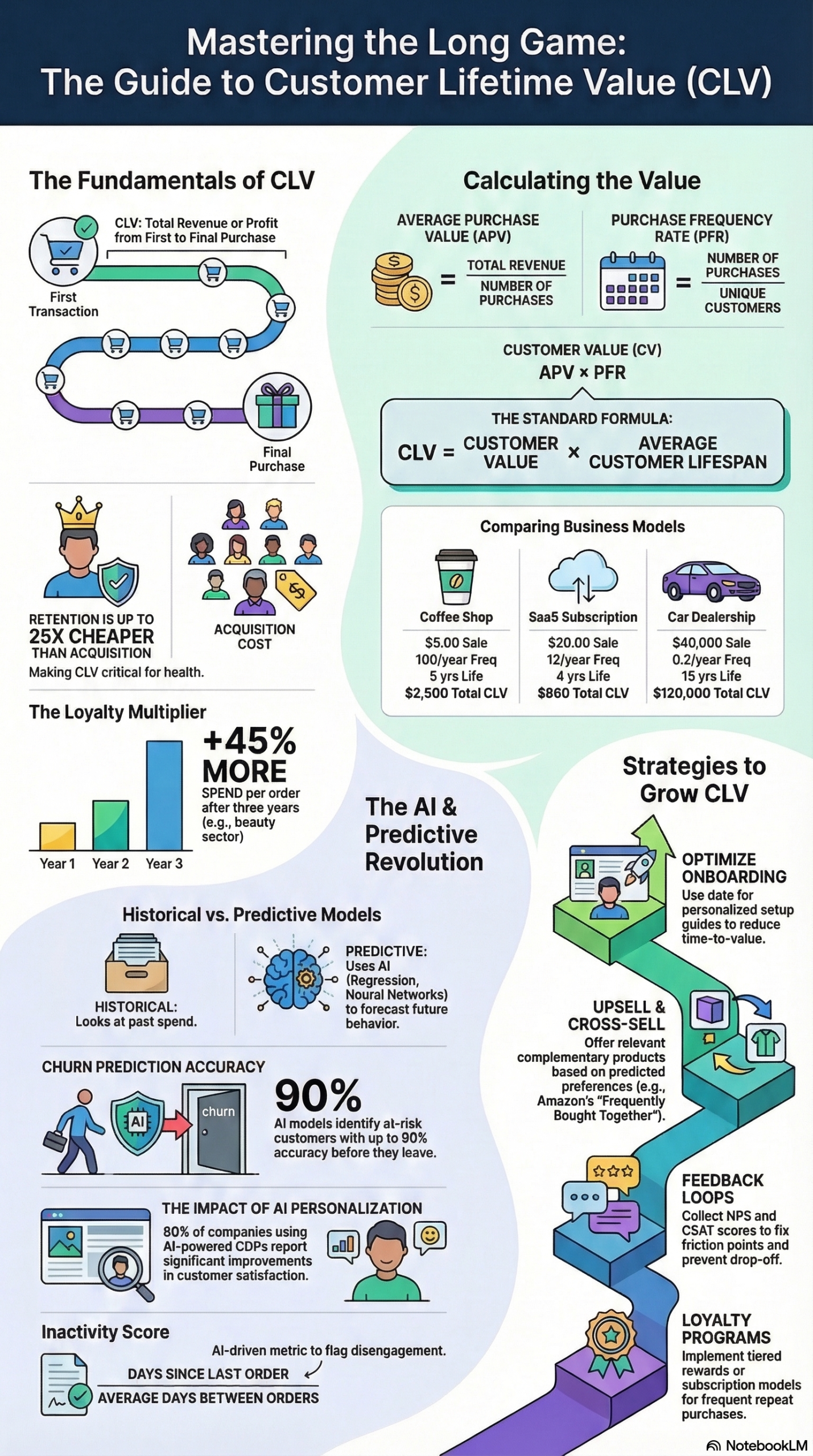
- Average Purchase Value (APV): Total revenue divided by total number of purchases in a period. This is the mean transaction amount.
- Average Purchase Frequency Rate: Total purchases divided by unique customers in the same period. This tells you how often the average customer transacts.
- Customer Value: APV multiplied by purchase frequency rate. This is the average monetary contribution per customer per period.
- Average Customer Lifespan: Sum of all customer lifespans divided by total customers. How long, on average, does a customer stay active before churning?
- Basic CLV: Customer Value multiplied by Average Customer Lifespan. The baseline expected revenue from a single customer relationship.
These formulas come directly from the NotebookLM CLV research report and form the foundation for every more sophisticated model built on top of them.
The Two Model Types: Historical vs. Predictive
The fundamental fork in CLV methodology is whether you’re measuring what happened (historical CLV) or forecasting what will happen (predictive CLV). Historical CLV sums actual past transactions — reliable, auditable, but inherently backward-looking. Predictive CLV uses historical data plus machine learning algorithms to forecast future buying behavior.
As Neil Patel notes, predictive CLV is where the real leverage lives: it lets you identify at-risk customers before they churn, flag high-potential customers for prioritized investment, and set maximum-acceptable CAC thresholds by segment rather than across your entire customer base.
Why Customer Lifetime Value Matters
The case for CLV as a primary business metric is not philosophical — it’s mathematical. Frederick Reichheld at Bain & Company quantified it: a 5% increase in customer retention rates can increase profits by 25% to 95%. That asymmetry is what makes CLV optimization one of the highest-leverage activities in any marketing budget.
Neil Hoyne, Chief Measurement Strategist at Google, has called CLV “the indispensable measure for marketers” — and from a practitioner standpoint, the reason is clear. CLV makes three things possible that no other metric can:
1. Rational Budget Allocation: When you know a customer segment has a CLV of $2,400, you can justify spending up to $800 to acquire them (maintaining a 3:1 CLV:CAC ratio) without guessing. Without CLV, acquisition budgets are set by feel or industry benchmarks that may not apply to your business model.
2. Churn Intervention Before It Happens: Predictive CLV models using AI can flag customers who are statistically likely to churn 30-60 days before they do, based on behavioral signals like declining engagement, missed repurchase windows, or dropping order frequency. That window is the difference between a retention campaign that works and a win-back campaign that’s too late.
3. Segmentation That Actually Drives Behavior: Not all customers deserve the same investment. The research report on CLV identifies three distinct response strategies: high-value customers get priority support, exclusive loyalty perks, and early product access; at-risk customers trigger automated re-engagement workflows; low-value customers are routed to efficient self-service channels. This tiered model prevents the common mistake of spending enterprise-level support resources on customers who will never generate enterprise-level revenue.
For marketers specifically, CLV reframes the entire conversation around paid acquisition. It converts “is this campaign profitable?” into “is this campaign acquiring customers who will be profitable?” — a meaningfully different and much more strategically useful question.
The Data: CLV Benchmarks by Business Model
Understanding CLV in isolation is limited. What makes the metric actionable is benchmarking it against acquisition costs and across industry verticals. The following tables draw from the CLV research report and Neil Patel’s CLV analysis.
CLV Formula Reference Table
| Metric | Formula | Example Output |
|---|---|---|
| Average Purchase Value (APV) | Total Revenue ÷ Number of Purchases | $47.50 per transaction |
| Purchase Frequency Rate | Total Purchases ÷ Unique Customers | 4.2 purchases/year |
| Customer Value | APV × Purchase Frequency Rate | $199.50/year |
| Average Customer Lifespan | Sum of Lifespans ÷ Total Customers | 3.8 years |
| Basic CLV | Customer Value × Avg Lifespan | $757.80 |
CLV by Industry Vertical
| Industry | Avg Transaction | Frequency | Lifespan | CLV |
|---|---|---|---|---|
| Coffee Shop | $5 | 100x/year | 5 years | $2,500 |
| SaaS Subscription | $20/month | 12x/year | 4 years | $960 |
| Car Dealership | $40,000 | 1x/5 years | 15 years | $120,000 |
| E-commerce (mid-market) | $65 | 3.5x/year | 3 years | $682.50 |
Source: NotebookLM CLV Research Report
CLV:CAC Health Check
| CLV:CAC Ratio | Signal | Action |
|---|---|---|
| 5:1 or higher | Strong unit economics; possible under-investment in growth | Increase acquisition spend in proven channels |
| 3:1 | Healthy benchmark for fast-growing companies | Maintain current strategy; optimize by segment |
| 2:1 | Margin pressure beginning | Audit acquisition channels; increase retention investment |
| 1:1 or below | Unsustainable — every customer costs as much as they generate | Pause scaling; restructure offer or churn rate |
Source: NotebookLM CLV Research Report
Step-by-Step Tutorial: Building a Predictive CLV Model
This walkthrough covers how to implement a full predictive CLV model — from raw transaction data to segmented audiences you can activate in a CRM or CDP. I’ll use Python with the lifetimes library, which implements the BG/NBD and Gamma-Gamma probabilistic models documented in the research report.
Prerequisites
- Python 3.9+ with
pandas,lifetimes, andmatplotlibinstalled - Transaction history with at minimum: customer ID, transaction date, transaction amount
- At least 120 days of historical data (the minimum required for model training, per the CLV research report)
- Access to your CRM or CDP for segment activation
pip install lifetimes pandas matplotlib scikit-learn
Phase 1: Prepare Your Transaction Data
Your raw data needs to be transformed into a customer-level summary table before any modeling can begin. The BG/NBD model requires four fields per customer: frequency (number of repeat transactions), recency (time between first and last purchase), T (total observation time), and monetary value.
import pandas as pd
from lifetimes.utils import summary_data_from_transaction_data

# Load your transaction data
df = pd.read_csv('transactions.csv', parse_dates=['transaction_date'])

# Ensure clean data — remove duplicates, standardize formats
df = df.drop_duplicates()
df['transaction_date'] = pd.to_datetime(df['transaction_date'])

# Build the RFM summary table
# observation_period_end = the last date in your dataset
rfm = summary_data_from_transaction_data(
    df,
    customer_id_col='customer_id',
    datetime_col='transaction_date',
    monetary_value_col='order_value',
    observation_period_end='2026-03-20'
)

print(rfm.head())
The output is a DataFrame with one row per customer containing: frequency, recency, T, and monetary_value. This is the foundation for both models.
Data Quality Check: Before proceeding, audit for common issues. Customers with frequency = 0 are one-time buyers — they’re valid inputs but require special handling. Negative monetary values (returns, refunds) should be zeroed out or excluded depending on your return rate. Cross-domain data (e.g., in-store POS combined with online orders) must be mapped to a single customer ID; the research report explicitly calls out this cross-domain mapping step as critical to model accuracy.
Phase 2: Train the BG/NBD Model for Transaction Prediction
The Beta Geometric / Negative Binomial Distribution (BG/NBD) model predicts how many future transactions a customer will make and estimates whether they’re still “alive” (active) or have churned. Unlike simple averaging, BG/NBD accounts for the heterogeneity in your customer base — it recognizes that some customers naturally buy rarely but reliably, while others buy in bursts.
from lifetimes import BetaGeoFitter

# Initialize and fit the model
bgf = BetaGeoFitter(penalizer_coef=0.0)
bgf.fit(
    rfm['frequency'],
    rfm['recency'],
    rfm['T']
)

# Predict expected purchases in the next 52 weeks (1 year)
rfm['predicted_purchases_1yr'] = bgf.conditional_expected_number_of_purchases_up_to_time(
    52,  # weeks
    rfm['frequency'],
    rfm['recency'],
    rfm['T']
)

# Calculate "predicted alive" probability
rfm['p_alive'] = bgf.conditional_probability_alive(
    rfm['frequency'],
    rfm['recency'],
    rfm['T']
)

print(rfm[['frequency', 'recency', 'predicted_purchases_1yr', 'p_alive']].head(10))
The p_alive score corresponds directly to the Predicted Alive Score described in the research report — an AI-generated metric determining whether a customer is still active or has likely churned. Any customer with p_alive < 0.4 is a priority for re-engagement.
Phase 3: Train the Gamma-Gamma Model for Revenue Prediction
The Gamma-Gamma model estimates the monetary value of future transactions for each customer. It assumes that transaction value varies randomly around a customer’s mean, and that the mean itself varies across customers. Combined with BG/NBD, it produces a full CLV forecast.
from lifetimes import GammaGammaFitter

# Filter to repeat customers only (frequency > 0)
returning_customers = rfm[rfm['frequency'] > 0]

# Fit the Gamma-Gamma model
ggf = GammaGammaFitter(penalizer_coef=0)
ggf.fit(
    returning_customers['frequency'],
    returning_customers['monetary_value']
)

# Calculate predicted CLV for the next 12 months
# Assuming a monthly discount rate of 1% (12.7% annually)
rfm['predicted_clv_12mo'] = ggf.customer_lifetime_value(
    bgf,
    rfm['frequency'],
    rfm['recency'],
    rfm['T'],
    rfm['monetary_value'],
    time=12,          # months
    discount_rate=0.01
)
You now have a predicted_clv_12mo column for every customer — the estimated revenue each will generate in the next 12 months. This is the Predicted Future Value metric referenced in the research report as a key AI-driven CDP attribute.
Phase 4: Calculate the Inactivity Score
The Inactivity Score is one of the most practical churn signals in the research. Per the CLV report, it’s calculated as: days since last order divided by that customer’s personal average days between orders. A score above 100 means the customer has exceeded their typical buying cycle — a strong churn signal.
# Calculate average days between orders per customer
customer_avg_gap = df.sort_values('transaction_date').groupby('customer_id').apply(
    lambda x: x['transaction_date'].diff().dt.days.mean()
).rename('avg_days_between_orders')

# Days since last order (as of observation end date)
last_order = df.groupby('customer_id')['transaction_date'].max()
observation_end = pd.Timestamp('2026-03-20')
days_since_last = (observation_end - last_order).dt.days.rename('days_since_last_order')

# Merge and calculate inactivity score
inactivity = pd.concat([customer_avg_gap, days_since_last], axis=1)
inactivity['inactivity_score'] = (
    inactivity['days_since_last_order'] / inactivity['avg_days_between_orders'] * 100
)

rfm = rfm.join(inactivity['inactivity_score'])
Phase 5: Segment Customers and Activate
With CLV predictions in hand, tier your customers into actionable segments for CRM activation. The research report recommends three primary tiers:
def assign_segment(row):
    if row['predicted_clv_12mo'] >= rfm['predicted_clv_12mo'].quantile(0.75):
        return 'High-Value'
    elif row['inactivity_score'] > 100 or row['p_alive'] < 0.4:
        return 'At-Risk'
    else:
        return 'Standard'

rfm['segment'] = rfm.apply(assign_segment, axis=1)
segment_summary = rfm.groupby('segment')[['predicted_clv_12mo', 'p_alive']].mean()
print(segment_summary)

# Export for CRM upload
rfm[['segment', 'predicted_clv_12mo', 'p_alive', 'inactivity_score']].to_csv(
    'clv_segments.csv', index=True
)
Upload clv_segments.csv to your CRM or CDP. In Salesforce, HubSpot, or Klaviyo, these segments map directly to list filters that can trigger automated workflows: retention sequences for At-Risk customers, VIP perks for High-Value customers, and standard nurture for the remainder.
Expected Outcomes: A properly trained BG/NBD + Gamma-Gamma model on 12+ months of clean transaction data typically produces CLV estimates with 70-85% accuracy at the segment level. Individual customer predictions have higher variance, which is why segment-level activation (not one-to-one targeting) is the right use case for this model.
Real-World Use Cases
Use Case 1: E-Commerce Replenishment Automation
Scenario: A DTC skincare brand has 40,000 customers across three product lines. Average repurchase cycle is 45 days. They have no systematic way to identify who’s about to lapse.
Implementation: Train BG/NBD on 18 months of order data. Flag any customer with an Inactivity Score above 100 as a triggered workflow entry. Klaviyo sequence: Day 1 — personalized reminder email with reorder link; Day 5 — limited-time free shipping offer; Day 10 — “Are you running low?” SMS.
Expected Outcome: Re-engagement campaigns triggered by behavioral timing (inactivity score) consistently outperform time-based blast campaigns because they reach customers at their natural repurchase moment, not an arbitrary calendar date. The research report notes that at-risk triggers like these are a core use case for AI-driven CLV.
Use Case 2: SaaS Churn Prediction and Expansion Revenue
Scenario: A B2B SaaS platform has 1,200 accounts ranging from $99/month to $2,000/month. Expansion revenue (upsells) represents 35% of total growth but is currently assigned reactively based on sales rep relationships.
Implementation: Build a predictive CLV model using subscription revenue data plus product usage signals (feature adoption rate, login frequency, support ticket volume). Accounts in the top CLV quartile with high feature adoption scores are flagged for proactive expansion outreach. Accounts in the top CLV quartile with declining feature usage are flagged for customer success intervention before renewal.
Expected Outcome: Per the research report, identifying which SaaS features correlate with long-term retention — then driving adoption of those features in the first 90 days — is one of the most impactful CLV levers available to product and CS teams. Combining CLV prediction with feature usage data creates a compound early-warning system.
Use Case 3: Paid Acquisition Budget Optimization
Scenario: An agency managing Google and Meta ads for a retail client is hitting ROAS targets but the client is concerned that profitability is declining quarter over quarter.
Implementation: Calculate historical CLV segmented by acquisition channel (Google Brand, Google Shopping, Meta Prospecting, Meta Retargeting). Compare CLV by channel against CAC by channel. The research report sets 3:1 as the healthy CLV:CAC benchmark for fast-growing companies. Any channel running below 2:1 is flagged for budget reallocation; channels above 4:1 are candidates for increased investment.
Expected Outcome: ROAS optimization and CLV optimization often produce different budget allocations. A channel with lower ROAS but higher average customer lifespan may be acquiring significantly more valuable customers. This analysis typically reveals 2-3 budget shifts that improve long-term profitability without reducing top-line revenue.
Use Case 4: Loyalty Program Architecture
Scenario: A regional coffee chain is redesigning their loyalty app and needs to decide which rewards to offer at which tiers.
Implementation: Segment customers by CLV quartile. Analyze which behaviors (visit frequency, average spend per visit, referral activity) correlate with high CLV. Design loyalty tiers that reward and reinforce those specific behaviors — not just total spend. Per the research report, Dropbox’s referral-for-storage model is a canonical example: the reward (extra storage) directly drives the behavior (more file uploads) that increases product stickiness and CLV.
Expected Outcome: Loyalty programs designed around CLV-driving behaviors outperform points-for-spend programs because they change customer behavior rather than just rewarding it.
Common Pitfalls
1. Training on Insufficient Data
The research report specifies a minimum of 120 days of historical transaction data for model training. Teams routinely attempt to build CLV models on 30-60 day datasets, producing predictions that overfit to seasonal patterns or recent anomalies. If you don’t have 120+ days of clean data, use historical CLV (backward-looking) rather than predictive CLV until you’ve accumulated enough history.
2. Ignoring Data Quality
The research report is unambiguous: “AI accuracy is entirely dependent on data integrity.” Duplicate customer records, inconsistent date formats, unmerged cross-channel identities, and unfiltered returns will systematically bias CLV predictions. Allocate 30-40% of your implementation timeline to data auditing before you touch a model.
3. Confusing CLV with ARPU
Average Revenue Per User is a population-level average. CLV is a customer-level prediction that accounts for differential lifespan. A business with identical ARPU across two cohorts but different churn rates has dramatically different CLV profiles for each cohort. Treating them as equivalent leads to misallocated acquisition spend.
4. Optimizing CLV Without Tracking CAC
Per the research report, CLV is most strategically powerful when paired with Customer Acquisition Cost. Maximizing CLV in isolation can lead to retaining customers who cost more to serve than they generate — especially in high-touch B2B environments. Always evaluate CLV:CAC together.
5. Running Static Models
CLV models decay. Customer behavior shifts with market conditions, competitive entries, and seasonal patterns. The research report recommends “Train & Predict” cycles run weekly or monthly to keep predictions current. A model trained once and never retrained will produce increasingly stale — and increasingly misleading — segment assignments.
Expert Tips
1. Use Cohort Vintage Analysis Before Modeling
Before building any predictive model, plot retention curves by cohort month. This reveals whether your business has a structurally improving or declining CLV trend — critical context for interpreting model outputs. A model trained on a deteriorating cohort will under-predict CLV for recent cohorts if the trend has reversed.
2. Incorporate NLP-Based Sentiment Signals
The research report notes that NLP analysis of customer emails, reviews, and support tickets can adjust predicted CLV based on emotional state and satisfaction level. A customer with a strong transactional CLV score but declining support sentiment is a churn risk your quantitative model alone won’t catch. Integrate support ticket sentiment (positive/neutral/negative) as a feature in your model.
3. Set Segment-Level CAC Maximums, Not Account-Level
Use CLV predictions to set maximum acceptable CAC thresholds by segment — not for individual customers. The research report is explicit: predictive CLV “allows teams to set maximum acceptable CAC for different customer segments.” This is operationally practical (you can implement it in your ad platform’s bid strategy) in a way that customer-level thresholds are not.
4. Prioritize First-90-Day Activation
The research report identifies the first 90 days as a critical CLV window for SaaS businesses — the period in which you should drive adoption of features correlated with long-term retention. The same principle applies across business models: the onboarding experience sets the trajectory of the customer relationship. Instrument your onboarding funnel with CLV-correlated milestones.
5. Build for Privacy Compliance from Day One
The research report cites that 80% of consumers are more likely to engage with brands that prioritize data protection. GDPR and CCPA compliance is not just legal necessity — it’s a CLV lever. Customers who trust your data practices have higher engagement rates and longer lifespans. Build your CLV data pipeline with data minimization and explicit consent mechanisms from the start, not as a retrofit.
FAQ
Q: What’s the difference between CLV, CLTV, and LTV?
These terms are interchangeable in most contexts. CLV (Customer Lifetime Value) and CLTV (Customer Lifetime Value) are identical. LTV (Lifetime Value) is a shorthand that SaaS teams favor. Some analysts differentiate revenue-based LTV from profit-based CLV, but in common usage they refer to the same underlying calculation. Per Neil Patel’s CLV guide, the metric concept is consistent regardless of abbreviation.
Q: How much historical data do I need to build a predictive CLV model?
Per the research report, a minimum of 120 days of transaction history is required to train a BG/NBD model with meaningful accuracy. For most businesses, 12-24 months produces significantly better results because it captures seasonal patterns and natural buying cycles. If you have less than 120 days, use historical CLV (sum of actual past transactions) as a proxy until you’ve accumulated sufficient data.
Q: What’s a good CLV:CAC ratio?
The research report sets 3:1 as the standard benchmark for fast-growing companies. Below 2:1, margin pressure becomes significant. Above 5:1, you may be under-investing in acquisition relative to what your unit economics could support. The right target varies by industry, growth stage, and capital efficiency goals.
Q: Can I build a CLV model without data science expertise?
Yes, with limitations. Customer Data Platforms (CDPs) like Segment, Klaviyo, and Salesforce Marketing Cloud include built-in CLV prediction features that handle the modeling layer. These are substantially less customizable than building your own model but require no ML expertise to operate. The trade-off is accuracy and interpretability — black-box CDP predictions are harder to audit and optimize.
Q: How do I handle customers who’ve only made one purchase?
One-time buyers are valid inputs for CLV modeling but require different treatment. The BG/NBD model handles them natively — it assigns them a lower probability of future transactions but doesn’t exclude them. In practice, segment your single-purchase customers separately, identify what percentage convert to repeat buyers within 90 days, and use that conversion rate as a CLV multiplier for new customer acquisition evaluation.
Bottom Line
Customer Lifetime Value is not a reporting metric — it’s a strategic operating system for sustainable growth. The combination of historical CLV for accountability and predictive CLV for forward-looking decision-making gives you the full picture that acquisition metrics alone can never provide. With the BG/NBD and Gamma-Gamma models now accessible via open-source Python libraries, building a functioning predictive CLV model is a weekend project for any analyst with clean transaction data. The research report on CLV makes the economic case plainly: a 5% improvement in retention translates to a 25-95% increase in profits, per Frederick Reichheld’s research at Bain & Company. As AI-driven Customer Data Platforms continue to push predictive CLV into the reach of mid-market businesses, the competitive advantage will shift to whoever acts on these predictions fastest and most precisely.


0 Comments